Friday, December 13, 2013

Python Coding

        
As well as creating Raster, Geocoding, Spatial Analysis and Interoperability data for the Trempealeau county data I was also tasked with creating python scripts which we would utilize in order to make our own selective tools. In order to do this I had to use the different sources that were available to me in the form of python. Arc GIS has an integrated python coding system with arcmap 10.2 which was very innovative and functional while the python script that is available to use on the University of Wisconsin lab computers is the Win Python coding system, this is a free to use python scripting software that is open source which can allow a multitude of options. The differences between the two are minor but significant at the same time.


I found that the integrated python scripting system that is in ArcGIS is more user friendly and allows the coding to be seen almost instantaneous. This also allowed me to mess around with the tools that are in Arc Map at the same time to see how they will be affected by my script. When I would code in the Arc Map python script help options would appear that would help with my understanding of the code I was scripting. In the Win Python application I could pull a window up to create a script and run later, this allowed for a free flow of coding that could be edited on the fly and saved in order to create tools. Using both of these python coding scripts I was able to create the three basic scripts that would create tools that were beneficial to Arc GIS.


                This script actually runs a Euclidean distance tool. in the scrip if the extension is available it will run a EucDistance tool on the bike route and create a cell size of 100, it will then save this distance in my folder as a new layer that I can use.


import arcpy

... from arcpy import env

... env.workspace = "H:/Documents/Esripress/Python/Data/Exercise05”

... if arcpy.CheckExtension ("spatial")=="Available":

...     arcpy.CheckOutExtension("spatial")

...     out_distance = arcpy.sa.EucDistance ("bike_routes.shp", cell_size = 100)

...     out_distance.save("H:/Documents/Esripress/Python/Data/Exercise05/Results/bike_dist")

...     arcpy.CheckInExtension("spatial")

# I left the below part out, if I tried to include it in the python script it would only return with Syntax Errors

>>>...     else:

...         print "spatial analyst license is not available."


                This next script that I created was a great undertaking as my coding was only in html before and that was during high school. So I was pretty rusty, however using the integrated python script in Arc Map I was able to create a code that would take a coordinate notation and that was incorrect and then project a correct coordinate system. In this case it took the Michigan coordinate system "Random_mi_project1" and converted it to the correct notation using the code arcpy.convertcoordinatenotation_management I then told it to project the coordinate system into UTM zoning, thus creating a correct coordinate notation.


Final Script to convert to UTM


#This is telling python to import arc python into the script. it is also setting the environment workspace

Import arcpy

from arcpy import env


Env.Workspace=”W:/geog/CHupy/geog337_f13/Kerraj/ex.#1”

#This is the code that is creating the new coordinate notation, it is switiching the notation from the incorrect notation into the correct UTM coordinates


arcpy.ConvertCoordinateNotation_management("random_mi_project1","H:/documents/arcgis/default.gdb/randomconvertutm", "POINT_X","POINT_Y","DD_2","UTM_ZONES","","")


# This is the final result that can be found


<Result 'H:\\documents\\ArcGIS\\Default.gdb\\randomconvertutm'>


This code allows me to print both the field class of a feature class as well as the shapes that they represent. To do this I used the append feature that allowed me to enter my own messages to the counties, polygons, and points. I marked Railroads, Counties and Cities as points, Lines, and Polygons that when told to print would print the name and type of shape file it is. I also used the field list to print the fields that they represent. This code is helpful to know because it lists all the feature classes that are as points, lines, and polygons. for example if I was curious to know what the points are I could use this script to find out that the points are cities. I can then use other codes to print out a list of the cities in the form of points and change the titles. I can also go and my own points and feature classes using this script, for example I could say points=["cities.shp","towns.shp"] and the points will be written that towns and cities are points.


import arcpy

from arcpy import env

env.Workspace= "H:/documents/esripress/python/data/exercise06"

# fclist is the feature class list, what I am telling python to do is to create a list of feature classes based on the list of "fclist"

fclist= arcpy.ListFeatureClasses()

print fclist

Lines= ["Railroads.shp"]

Polygons= ["Counties.shp"]

Points=["Cities.shp"]

Points.append("Are all point feature classes")

Lines.append("Are all line feature classes")

Polygons.append("Are all polygon feature classes")

print Points

print Lines

print Polygons

fieldlist= arcpy.ListFields("Railroads.shp")

fieldlist= arcpy.ListFields("Counties.shp")

fieldlist= arcpy.ListFields("Cities.shp"]

for field in fieldlist:

    print field.name + ""+ field.type


                This code allows me to create a feature point class that only allows the points to exist that only have the attribute of having Sea Plane Bases inside the attribute table. This allows me to select points based on attribute table data, for example, Sea Plane Bases. I can then use this code to create a buffer around the sea plane bases to create a buffered base, in this case I took the sea plane bases and created a buffer of 7500 meters from the buffer_analysis script tool.


import arcpy

from arcpy import env

env.workspace= "H:/documents/esripress/python/data/exercise07"

import arcpy

from arcpy import env

env.workspace= "H:/documents/esripress/python/data/exercise07"

infc= "airports.shp"

outfc= "results/airports_seabases.shp"

delimitedfield= arcpy.AddFieldDelimiters(infc, "FEATURE")

arcpy.Select_analysis(infc, outfc, delimitedfield+ " = 'Seaplane Base'")

fc= "airports_Seabases.shp"

unique_name= arcpy.CreateUniqueName("Results/seaplanebuffer.shp")

arcpy.Buffer_analysis(fc, unique_name, "7500 METERS")

fc= "airports.shp"

unique_name= arcpy.CreateUniqueName("Results/buffer.shp")

arcpy.Buffer_analysis(fc, unique_name, "15000 METERS")


Raster Dataset Modeling and Suitability


Our goal for this blog post is to use rasters to convert a message that what mines would be both suitable and environmental to the county of Trempealeau Wisconsin. We will be assessing the risks involved with mines in proximity of schools, lakes, and other important features. The risks associated with mining are great. Mining can cause a vast array of ecological and human hardships in the form of water pollution, air pollution, and erosion. in order to combat these three big three hardships we will be using the raster modeling to look at the slope of the selected mining areas and of the water close to the selected mining areas. When we know the areas that would be less optimal to set a mine on we can then select an area that will minimalize the effects of mining on the environment. This is called the risk model. We will use this model in order to pick an area that offers the lowest amount of risk to the mining operation as well as to the environment.


We will also have to look at the area that we are mining. We will want an area that is both high in frac mine sand and in a fairly easily accessible area to mine. The more excessive mining techniques that we have to utilize in order to mine frac sand will increase the amount of cost to the mining companies. We will want to select a mine that is easily accessible via rail roads or roads in order to cut down on transportation costs. We will also have to look at what kind of soil or land type that we are going to be mining in. Rocky areas and heavily treed areas as well as wet lands are not appropriate nor cost effective to mine so we will have to look at shrub land farrow land and other grassland areas. Another focus will have to be looking at cropland to mine since this is already developed land that is easily accessible. we will also have to look at the proximity these areas are in with developed land where people live as well as water sheds. This is called a Suitability model and we will use it in order to select a good area to mine that will both be productive and cost effective.

   In order to start out with this project will only be using part of Trempealeau county data otherwise the vastness of the county will dwarf the area. To start the suitability model I used the boundary function clipped with the Geology to create a smaller version of the Trempealeau county data. This smaller version of the Trempealeau county data will be easier to manage and will allow a faster area to materialize for mining data. From this point we will have to select data that is needed for mining. The two most desirable areas for geologic sand mining are the Jordan and Wonewoc formations. In order to create a raster from these formations I took the TMP Geology layer and created a raster with the "Feature class to raster using table tool" The table that I used to create the raster was the Geology unit field. This field holds the Jordan and Wonewoc features. When the raster was created I used a re-class tool that I made in Model Builder to create a ranking with Wonewoc formation as the top since it has the greatest amount available, I Then used the Jordan as the second rank since there was less and it was closer to water areas the final rank I assigned was for all the data that we did not want on our model.


This is the selected Geological areas in raster format
I Selected Wonewoc as the top rank and Jordan as the 2nd choice
due to the lack of mining oppurtunities that Jordan offers.


In order to use the geological raster in conjunction with our other rasters we need to find out what kind of land cover we have on the map and what is the best choice to choose for a sand mining location. In order to do this we need to go to the NLCD website to download the NLCD (National Land Cover Data) so we know exactly what is cover the Trempealeau County. The things that we need to think about is how much effort will we have to do on the land in order to extract the frac sands. For my top rank I chose Clover, Wildflowers, Seed, Sod grass, and other pasture/hay NLCD cover, this will allow for the easiest mining area and is more abundant than the second rank which is shrub land and grasslands which is not owned by farmers or other private parties. For the last rank I selected all farm land that is not a tree farm in order to allow ease of mining. The reason why I selected wild grassland over farm land was because it will allow ease of mining and it will not displace any farmers, avoiding bad press and the already controversial issue of frac mining in Wisconsin. I selected Pasture land as my top selection mainly because the amount that is available in Wisconsin as well as the ease of mining. It however, may displace farmers but you have to crack a few eggs in order to make an omelet. I believe that this is a necessary risk that has to be taken in order to have the best mining area possible.

 
This is the Raster for the selected areas of Land Cover based on
NLCD criteria and on effort needed to clear the land to mine.
 

This is area that is unsuitable to mine based on NlCD criteria
it is mostly water, wetlands, tree cover and rocky areas.
these are not optimal nor cost effective to mine.
 

After I selected the Land cover that will be used to select an area that frac sand mining is possible I had to find the distance between the railroad loading stations and the distance between the optimal land that I had to use. For this I used the Euclidean Distance tool on the rail depots as this allows us to know the distance to the closest loading station. The problem that I encountered was when I went to convert the feature point to a Euclidean Distance it would result in errors. To combat this problem I went and took my final rail loading mines merge from exercise 7, which contained the loading stations for frac mines to rail stations, and converted it to a raster using the tool Point to Raster. With this new raster I could use it as a source cell for the Euclidean Distance tool to use. I set the Euclidean Tool to 5000 meters, anything in this area would be optimal for a mining operation, of course the closer to the center the better. This is useful to know because the less travel that the mining operations have to make to a rail station is money that is saved that can be used for other more important things, this also allows for a larger profit.


Selected Euclidean Distance of Rail Loading Terminals


After the Euclidian distance tool was ran I then had to find out the suitable slope that will be used to have the optimal mining criteria. Slope is important to note when it comes to mining as if you do not take into account of the slope it could lead to ecological problems such as run off and erosion. This can turn into a health hazard as the run off can come into contact with a watershed or a river. This could turn into an ecological disaster and is probably best to be avoided. To find the suitable land slope I used the old Trempealeau county data geodatabase from exercise four and used the DEM to calculate the slope. I had to change it from ft. to meters in order to have the output show correct values and I used the filter tool to create a mean average of the slope that is used in the Trempealeau county data. This is set in a 3x3 cell size in order to create the average slope throughout Trempealeau county. I then used this data to create a new layer based on the average slopes that I thought would allow the easiest and most accessible areas for mining. I chose the mean averages to reclassify in order to have the easiest access for mining. I excluded the lowest points and the highest points as the lowest would have run off into the mining areas that could hamper operations, I excluded the highest points as it would be difficult to mine those areas. I used the reclassify tool to exclude the two highest points and two lowest points to accomplish the slope suitability areas that you can see below.


Suitable Slope that can be mined


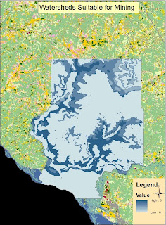
Water depth is an important criteria when it comes to sand mining as although it may be in our best interest to try not to be close to pollute water systems we still need water in order to lubricate the drill for mining.  I had to use a generalized water table elevation map for Trempealeau county for a good location to mine which I downloaded at wisconsingeologicalsurvey.org we then had to use this coverage data and convert it to a raster. To do this I converted it from coverage data to a raster using the topo to raster tool.  It takes topological data and converts it to a raster format we are using it in this format as the contours data can be subjected to a raster format. I had to use the large boundary surface in order to convert the contours into a raster format. Once the contour data was converted into raster I clipped the data with my Trempealeau County base layer. Once I had a suitable raster I then used my Reclass tool based on areas that would allow a better mining area to be found based on my criteria.


Watershed Suitablilty model

Finally once I have all these rasters it was time to create a sustainablility raster. To do this I combined all the rasters into one resulting index model. I then had to exclude all the data that I cannot use in our raster format. once we removed all the excluded lands we finally have our final product. A sustainability Raster for the best areas in Trempealea county to mine.


Sources:
 http://wisconsingeological survey.org/gis.htm
http://www.mrlc.gov/nlcd01_leg.php


Tuesday, December 3, 2013

Network Analysis


The goal of this project is to create a network analysis about the truck traffic that will happen on the Wisconsin roads from the excess traffic created from the frac sand mines. We can also calculate roughly the amount of money that it will implement on the counties from the extra road traffic. The network analysis model that is created will show the shortest distance from the mines to the mine distribution rail system


To begin this exercise I imported the base map of Wisconsin as well as topographic data and county data. I overlaid the county data and made it transport while keeping the outline opaque in order to create a see through version of the counties without having to extract a second layer. I did however create an attribute layer of just Trempleau county since this is an area of interest. From here I started the network analyst tool. I had to set the mines as incidents and the rail loading terminals as facilities since the mines will be going towards the facilities not facilities to mines. From here I had Arc Map solve the closest distance between the mines and the loading terminals.
 
This represents the incidents and facilities
in a network analyst map.
the quickest route from incidents to facilities is in yellow.

I also created a data model out of Data Model builder to build a network analyst quickly that can be used over and over again. This data model uses the same tools from ArcGIS that can be used separately with the same result however this allows the data model to be implemented multiple times and can be edited to suit different needs. Here I have it creating the best possible route from the frac mines to the rail distribution centers.

The Data model to create the quickest route


The results from the model builder.
note that this model builder includes all facilities and incidents
this will require some editing to remove the unneeded facilites and incidences

This is the final product that results from the use of my data model and from the network analysis of the county data and frac mines. We can see the quickest route and have a total distance in the form of time measurement. We can also calculate the amount of damage that the extra truck traffic is having on the county roads.
 

 These are the three final maps that I created using the Network Analyst tool and Model Builder
 
 This map showcasees all the frac mines to the distribution plants
This network analyst map showcases the Truck routes that will pass through
Trempealeau County on their way to a distribution rail system.
with this map we can calculate the total cost that was placed on the roads of
Trempealeau county.

 This is the final map showing all the quickest routes from the frac mines
to the distribution rail systems.

The results that are from the network analyst map shows the quickest route from the mines to the distribution plants. the way that this is significant is that it shows the quickest route and hence it is the cheapest route that the mine would be interested in making since it will cut into the profit margin less. This also shows the total amount of road maintenance that a frac sand mine may have on a county so they can be taxed to offset the amount of damage that the heavy truck traffic will have on the road systems.

 The total amount of cost for all of the routes in wisconsin
calculated using the ArcGIS network analyst tool.
 Using the total time coluom in the Trempealeau county data we can
calculate the total cost on the roads from the frac mine routes.
 

Using ArcGIS and Network analyst with model builder we can create a many multi layered projection of the quickest routes from frac mines to the rail distribution centers. This also allows us to calculate the total distance and we can then in turn create a projected cost that the trucks will have on the roads. This shows how powerful of a tool network analyst can be.

Monday, October 28, 2013

Geocoding


For this assignment we were tasked to download data from a county website and using that data connect to a database server and then geocode the data from the excel file found on the county website. The data that we used came from the Tremplealeau county land records. After downloading the starting geo-database from the trempealeau county web servers it became apparent that the records that were on file were all In different forms of measurement; for example we had data that would read as north sector 22 and“about a ¼ mile down country road M” this is data that we could not use in our mapping of the frac mines and would have to be normalized into correct address labels such as a street address. There were a total of about 132 total sand frac mines that were needed to be geocoded so instead of geocoding every sand mine the task was broken up into 22 separate areas so we were only tasked to map 14 – 18 by ourselves. These 14-18 geocoded points were then transferred into a geo-database and were used to show all the sand frac mines  operational in Wisconsin.


Normalizing data is the process of taking the unusable data and making it usable. The reason why we have to do this is because when the data came to us instead of having it in a usable format such as a street address it came to us in a jumble of coordinates and addresses. An example is that we had PLSS coordinates mixed with regular street addressess, this made it so that the geocoder could only geocode a couple of the addresses. The ones that were in the right spot were the ones with the regular street addresses. Knowing this we could then manually map the remaining missing addresses.


This is an example of data that is not normalized
This is an example of data that came with the Trempealeau county Database

In order to map the frac sand mines we were required to geocode the addresses acquired from the tremplou county data. Geocoding is the process of taking data from an excel file or other similar file system and extracting that data into a usable format that we can use to map as points polygons or other features. This can lead to certain errors however such as inherent errors. Inherent errors are errors that are present in the data from the start. An example of an inherent error that I encounted while geocoding would be the age of the maps that we used. In Google Earth we could see that the sand frac mine is operational but in the arcgis basemap that I utilized it wasn’t even constructed. After I found the areas that I needed to geocode for the point of the frac mines it was time to normalize the data so we could have a usable address.


This is an example of an inherent error from the arcgis basemap
in this picture it shows that no develpoment has occured.


But in this newer satellite image we can see a frac mine has been developed 
 
In order to rectify the inherent errors I used the geocode tool bar in the arc gis mainframe to present our own addresses this can be done a number of ways, one such way would to insert a point yourself but the way I accomplished this task was importing a base layer that had all the addresses in it from the start, then using google earth I entered the closest address that was presented to us from the Trempealeau county data. This type of Geocoding is called "Fuzzy Matching," it uses a predetermined address based on a scale of accuracy from 0-100% that I could selectso little editing would need to be done in the excel file. This way however, can lead to operational errors which is error in the form of user error. For example in one case I mapped an error just outside of the sand frac mine but one other student in the class mapped the opposite side of the frac sand mine.

 
 This is the Trempealeau county data normalized into a format that we can use for Geocoding.


This is an example of operational error.
Notice the distance between the other students point (red dot)
and my point (Green Triangle)
because of this error there could be accruracy issues associated
 

When we compared data to the other members of the class I was happy to see that our output points were fairly close together. This means that all our points were accurately labeled with little operational error involved. I still came across some problems that were my own doing. When I started the project the data that we were using did not come with unique ID codes so the data that I had been working on did not have an ID that I could match to the other student’s data. When the geo-database was released to us to my dismay my points could not be selected in an attribute search. I rectified this problem by starting up editor and manually inserting a unique ID field into my attribute table and from here I manually inserted the unique Id into each one of my cells by looking up the unique id in the geo-database that was provided to us.
The Final map with Geocoding Frac Sand mines.


This mapping exercise was very beneficial to me as it allowed me to work with real world data with real world problems associated with the data. It also allowed me to test me mettle against working with inherent and operational errors that can be a cause of many problems, and headaches.

Wednesday, October 2, 2013


Open pit mining is a very controversial topic today in Wisconsin. This mining is called Sand frac mining and it is the process of digging for the fine silica sand that is used as a proppant to hold open cracks in the rock to extract oil and natural gas. Wisconsins sand is very high quality and not found anywhere else thanks to the glacier deposits from the Cambrian age over 500 million years ago. The frac sand mining has been especially heavy in the northern parts of Wisconsin especially in Barron and Chippewa County. This has caused a heated debate about the environmental damages that could result from heavy mining, including air pollution, water pollution and land pollution.

This particular issue has affected my family personally, We owned property that was located next to a parcel that was high in silica sand. A mining company that digs for silica sand bought the land next to us and systematically bought all the remaining land around our property until we were forced to sell before the value plummeted. Our family land became worthless as hunting land so we sold it to the company. You can see the frac mine that they built on my family’s old land with these long/lat coordinates

Latitude 45°22'11.57"N Longitude 92° 1'7.88"W

Silica sand is very pure and high quality sand that naturally occurs in Wisconsin, it is also a vital component in the process of hydro fracking.  Hydro fracking is the drilling process of digging a well under the ground and cracking the hard rock layer to expose natural gas and oil. Water, Chemicals and frac sand are then continuously pumped into the crack at high pressures in order to keep the crack open and allow the oil and natural gas to flow out easily.

The methods that are used to dig for frac sand involve removal and excavation techniques of the top soil, digging below ground water lines, and blasting to produce shot rock which is then crushed to extract silica sand. The sand is then shipped to processing plants where it undergoes washing, drying, screening and a resin coat to allow the sand to be water retardant and flow as a slurry. It is then transported to its final destination, transporting frac sand in Wisconsin is preferably done by train instead of trucks so that road deterioration is less of an issue.

The issues associated with Frac Sand mining are about the air pollution and water table pollution. Hazardous air pollutions are known to occur from sand mining and processing operations but the silica sand itself is safe, the methods that are used to dig for the sand however is liable to release elements into the air that can be hazardous to people’s health. Sand Mining can also be hazardous to the water tables since any site located near a river, stream, lake or wetland may come into contact with site products. The products of sand frac mining may also make its way into drinking water.

We will be using GIS to explore some of these issues with frac sand mining including mapping the railway tracks that are delivering sand to refinery’s and processing plants and also the sand frac mines themselves. With this information we can create topology layers and estimate the amount of run off that we can expect based on the amount of rainfall and the elevation. We can also create buffers around plants based on expected pollution and the amount that is allowed based on the Wisconsin Department of Natural Resources.